
Six famous YouTube trading methods coded as taught: zero edges, one blown-up account
A lineage of six studies that turned famous YouTube and course methods into code exactly as taught: a celebrity trend method, Granville's law with a 200 EMA, the DEG method, an Elliott wave-3 short, and a gold-only martingale EA giveaway. Almost everything tested out as no edge or a re-labeled known edge, and the giveaway EA destroyed the account in two months on its own disclosed settings.
“The 10-billion-yen trader.” “Win from zero.” “Gold-only, high win rate EA, free to download.” Over the past months I took six famous methods from YouTube videos and trading courses, coded each one exactly as taught, and measured it on real data. The punchline up front: zero new edges. Almost everything was either no edge at all or a re-labeling of an edge I already trade, and the giveaway EA, run on its own disclosed parameters, wiped out the account two months in.
This article gathers those six studies into one lineage. The goal is not to attack any video or author. It is to lay out, in plain numbers, what happens when you take the stated rules at face value and measure them.
First time here? What you need to know
For new readers: this blog is a verification diary. I (one person) build my own automated FX trading program (an EA), statistically test trading methods, and publish everything, wins and losses alike. “Study N” refers to my numbered research log. The tests run on about 11 years of real data across FX pairs, gold and stock indices.
Four terms. PF (profit factor) = gross profit over gross loss, above 1 means profitable. IS/OOS = splitting data into a rule-selection period (In-Sample) and an untouched answer-key period (Out-Of-Sample). Walk-forward = freezing the rules on past data, then scoring them on data they have never seen. bp (basis point) = 0.01%, used for average per-trade returns.
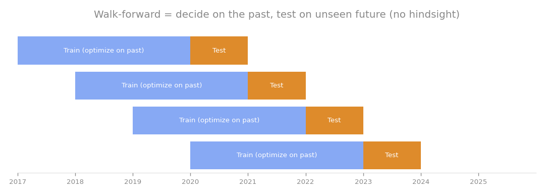
Walk-forward testing. All six methods faced the same arena.
The ground rules
Every study follows the same procedure. Take the rules the video or course actually discloses and translate them into code. Where the method needs human judgment (wave counting, line drawing), approximate it with something objective like an EMA slope, and say so openly. Eliminate any leak of future prices. Test on the same real data as everything else on this blog. Let the numbers decide.
“As taught” is the important part. No tweaks to make it win, no sabotage to make it lose. Here are the six, in the order I ran them.
Method 1: the “10-billion-yen trade” (study 54)
This is the approach of Ishin-no-suke, a well-known Japanese trading educator with books, a blog and a YouTube presence. The core is Dow-theory trend following: read the environment across multiple timeframes, then trade “four classic patterns” on the 4-hour chart, buying pullbacks, selling rallies, catching reversals. His exact moving-average settings sit behind paid material, so I mechanized the skeleton he discloses publicly.
The walk-forward results across eight currency pairs, fixed parameters, no hindsight:
| Variant | Total return | PF | Winning years |
|---|---|---|---|
| Long only | -2.9% | 0.96 | 4 of 10 |
| Pullbacks plus rally-selling (faithful) | -19.0% | 0.85 | 3 of 10 |
Notice that the version most faithful to the method, the one that also sells rallies, loses more. The author himself says trading is a game of skill, and that is consistent with what I measured: whatever earns money here lives in the discretionary layer of line drawing and crowd psychology, not in the mechanizable skeleton. The skeleton has no robust edge.
Method 2: Granville’s law with a 200 EMA, aiming for wave 3 (study 83)
A popular animated tutorial series teaches this one: in an uptrend, wait for price to pull back to the 200-period exponential moving average, then catch the third wave as it resumes. The wave recognition is subjective, so I approximated it with the EMA slope and implemented three entry modes: recross (price crosses back above a rising EMA), bounce (a bullish candle off the EMA touch), and deviation (a contrarian entry after a large stretch away from the EMA).
In-sample, all three modes landed at PF 0.96 to 1.01. That is essentially no edge before the real exam even starts. Walk-forward, the long-only recross made +5.6% and the long-only bounce +5.1%, but each won only 4 of 6 years, short of my robustness bar of 5 out of 6. Profits like that are the market’s upward drift, not the method. The contrarian deviation mode lost -25.4% with 2 winning years out of 6. A wipeout.
Method 3: the Matsuyama DEG method (study 102)
DEG blends Dow theory, Elliott waves and Granville into one video method: confirm wave 1 through breaks of a trendline, the Dow structure and the 20 EMA, then buy the Fibonacci retracement to ride wave 3 with a fixed risk-reward take-profit.
Of the six, this one came closest. The RR2 configuration went 6 winning years out of 6 in walk-forward testing. Then the robustness checks arrived. Shifting to RR2.5 or a 50-period EMA dropped it to 4 of 6, and merely changing the SMA period to 150 collapsed it to a -6.3% loss with 2 of 6. That kind of parameter sensitivity is the fingerprint of overfitting. The PF was a thin 1.09, and the correlation to my existing trend core measured 0.66. In other words, the machine version of DEG is a rediscovery of long trend following, not an independent edge.
Method 4: the Elliott wave-3 short, made objective (study 153)
A video series teaches a short setup: read the environment on the daily chart, then sell the 4-hour rally to catch Elliott’s third wave down. My objective version: daily close below the 200-day moving average, the 4-hour pullback rejected near its own 200 EMA, entry on the break of the rising support line. Two exit variants: target the measured length of wave 1, or exit when momentum fades (falling ADX or a shrinking MACD histogram). All inputs delayed to prevent leaks.
Results on six yen crosses, 4-hour chart:
| Period | Exit | PF | Monthly return |
|---|---|---|---|
| IS (2015-20) | Measured wave | 1.06 | +0.104% |
| IS (2015-20) | Momentum fade | 0.93 | - |
| OOS (2020-26) | Measured wave | 0.63 | -0.259% |
| OOS (2020-26) | Momentum fade | 0.74 | -0.081% |
A textbook case of overfitting: a slim in-sample profit that collapses to PF 0.63 on unseen data. Two things were still worth the effort. The momentum-fade exit cut the maximum DD (drawdown, the fall from an equity peak) from -16.4% to around -6%, a real defensive effect that nevertheless fails to produce a profit. And the study proved that supposedly unquantifiable judgment calls, line strength, wave structure, fading momentum, can in fact be quantified and tested. Being measurable and being profitable turned out to be different things.
Method 5: the gold-only martingale EA giveaway (study 238)
A promotional video offers a free “gold-only, high win rate” EA. The four-stage entry signal is secret, but the video discloses plenty: 300k yen starting capital at 0.04 lots, sizing up as profits accrue, an averaging-down grid spaced 50 to 250 pips (volatility-linked), take-profits of 4 to 13 pips, grid skipping in fast markets, vague stop-loss talk, and hedging once floating losses grow.
The three advertised logics unmasked: “irregularity evaluation” is a random-walk filter. “Liquidity distortion absorption” is the resolution of a multi-timeframe divergence; a proxy test does show +5.55bp on gold dip-buying, but that is a re-description of the gold long pullback my system already harvests, so nothing new. “Dynamic optimization” means the volatility-linked take-profit and grid spacing.
The engine simulation settles it. Running a grid faithful to the disclosed parameters on eleven years of 15-minute gold data, with a generous spread assumption, the account hits zero on 2015-03-10, two months after starting, holding up to eleven averaging-down layers. Scaled to a prop account, the worst single day is -101.92%. Whatever the secret entry signal is, a no-stop martingale money structure keeps the same distribution: a high win rate on the surface, total loss in the tail.
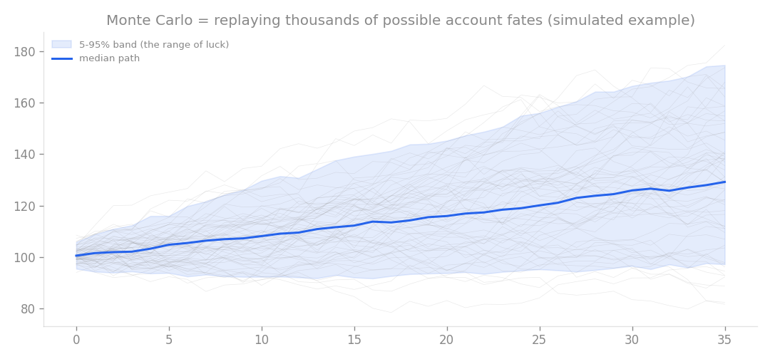
Judging an account by its distribution of fates. The rare total loss hiding behind a high win rate never shows up in the average.
Method 6: doubting my own study and re-measuring (study 238 addendum)
Then I called out my own work. Two of the three advertised logics had been dismissed by citing my older research, which breaks my measure-from-zero policy. So all three got re-measured on current data, every cell reported, no cherry-picking.
The irregularity filter went through a 40-cell sweep: trading only when the market looks “regular” consistently worsened the long side (a raw +5.65bp becoming -3.5bp after filtering), and the occasional good-looking cell flips sign between periods. The liquidity-distortion idea was compared against 200 random-timing controls within the same regime: the short side shows a genuine footprint (+4.04 vs +2.06bp, p=0.025), but it decays to a quarter out of sample and nets out to roughly zero after costs. Faintly real, unusable. The dynamic-optimization claim, that volatility-linked spacing suppresses drawdowns, got a head-to-head of three grid variants, and the video-faithful version with volatility linking and fast-market skipping blew up first, in March 2015, ahead of a fixed-spacing grid. The claim and the measurement point in opposite directions.
A rejection by citation leaves room for “but my settings are different”. A rejection by measurement closes that room. The verdict did not move; the quality of the evidence did.
Three patterns across all six
| Study | Measured essence | Verdict |
|---|---|---|
| 10-billion-yen trade | Walk-forward -2.9% / PF 0.96 (long only) | No robust edge |
| Granville 200 EMA | IS PF 0.96 to 1.01 | No edge |
| Matsuyama DEG | PF 1.09, collapses to 2/6 years on SMA 150 | Trend rediscovery |
| Elliott wave-3 short | OOS PF 0.63 / monthly -0.259% | Overfit |
| Martingale EA (engine) | Broke in 2 months, worst day -101.92% | Unusable |
| Same video, re-measured | All three concepts fail | Still no |
The first pattern: mechanized, everything converges to “go long and follow the trend”. Dow theory, Elliott waves, Granville, Fibonacci, in any combination, collapse into the same shape, leaving only a high correlation to the trend strategies I already run.
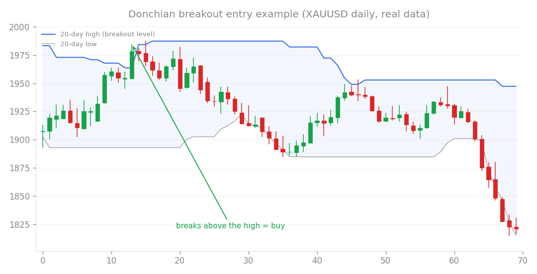
The convergence point. Strip the discretion out of a famous method and what remains is another paraphrase of riding a long trend.
The second: the earning power, if it exists, lives in the part that resists mechanization. The moment wave recognition or line drawing gets replaced by an objective proxy, the edge vanishes. That is not the same as calling the method fake. It is a precise statement: the rules as disclosed carry no edge.
The third: a high win rate can be manufactured by money management alone. A no-stop averaging-down grid shows you many small wins and hides the rare total loss in the tail. When someone advertises a win rate, ask what happens on the day it loses. That question is what six studies’ worth of tuition bought.
I do not claim any of these videos or courses are scams. I did not measure the discretionary skill of their authors, and I cannot reject what I cannot measure. I can say exactly one thing: coded as taught and measured on real data, none of the six left anything my system could adopt.
This article consolidates studies 54, 83, 102, 153 and 238.