
When should you buy a crashing stock? I tested 21 years of daily data on 613 tickers
It started with a hypothesis: buy stocks that crashed during the week at Friday's close, sell into the rebound. Friday turned out to be the worst possible day. The full story of seven studies, including the failures, the generalization tests, mark-to-market precision, and the survivorship stress test.
This all started with a reader-style request: test the idea of buying stocks that fell hard during the week at Friday’s close, then selling into the rebound once the market calms down. The verdict up front: the hypothesis was rejected, but it failed in the most instructive way possible. Buying crashes turned out to be right, and only the Friday part was wrong. Seven studies later (research notes 247 through 253), one crash-buying rule stood confirmed across 21 years and every market regime in the data.
It is a long article, because the detours and failures are the actual substance. In order, then.
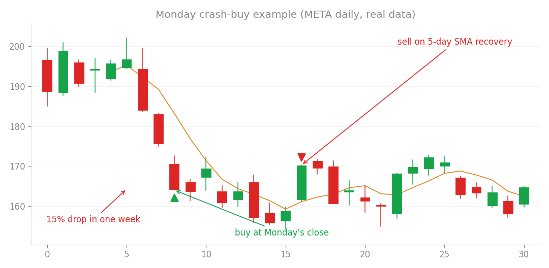
The final rule in action: META falls 15% in a week, gets bought at Monday’s close, and is sold on the 5-day SMA recovery.
The rig, and two breakwaters
Everything runs on US stock daily data, 429 tickers at first and 613 by the end, covering up to 21 years (2005-2026), with round-trip costs of 2 cents plus 2bp deducted from every trade.
Two forces routinely corrupt long-only stock studies. The first is bull-market inflation: in a rising market, everything “works”. So every test runs against 200 sets of random-timing entries in the same stocks with the same trade counts and holding periods; a strategy that cannot beat that control has no timing skill, only beta. The second is hindsight: adjust rules after seeing the data and you manufacture something that only ever worked in the past. So the data was split into 2005-2017 for rule selection and 2018-2026 as sealed out-of-sample (OOS), with kill criteria written down before testing.
These two breakwaters carry the credibility of everything below.
Chapter 1: Friday lost 25 times out of 25 (study 247)
First, the original idea, exactly as proposed: buy at Friday’s close when the weekly return breaches thresholds from -5% to -15%, with five exit types (5- and 10-day time exits, 5-day SMA recovery, half-retrace targets, wait-for-calm) and optional filters, 40 variants.
Crash-buying itself was strong: 25 variants passed the gates (N over 100, t over 2, PF over 1.15) and nearly all beat the random control at the 100th percentile. Then came the control that mattered: enter the identical crash signal on each weekday separately.
| Entry day | Avg return per trade (-5% crash, SMA5 exit) |
|---|---|
| Monday | +106.9bp |
| Tuesday | +43.3bp |
| Wednesday | +44.5bp |
| Thursday | +78.1bp |
| Friday | +14.8bp |
Friday came last in all 25 variants, significantly so (Welch t reaching -5.3). Friday’s close sits mid-panic, and the position eats the weekend follow-through, Monday margin calls included. The wait-for-calm instinct was correct; the waiting simply stopped one step early.
The pre-registered kill criterion fired and the hypothesis died. Bonus finding: the wait-until-volatility-calms exit was the weakest of the five. The heart of the rebound happens before things calm down.
Chapter 2: switching to Monday, and this time it held (study 248)
The weekday control pointed at Monday, so Monday became a freshly registered hypothesis. Full disclosure belongs here: this variant was born from looking at data, and sign-flipped derivatives have died on unseen data before in this project (an index gap strategy did exactly that). Hence the pass criteria were frozen first, and the sealed OOS years, 8.5 of them including the COVID crash and the 2022 bear, were appointed judge.
It survived.
- In-sample: 23 of 24 variants passed, and Monday concentration beat the any-weekday pool in every one
- Out-of-sample: the flagship (5-day return below -10%, buy the first close of the week, sell on SMA5 recovery) earned +120.4bp per trade, t=+9.1, PF 1.42
- It beat the random control at the 100th percentile and the any-weekday version by +41bp
All four pre-registered kill criteria cleared, making it this framework’s first-ever OOS survivor. The structural story is clean too: panic compresses into Friday’s close, the weekend digests the news, the last capitulation prints on Monday, and the reversion starts from there. Monday’s close is the first close after the selling has exhausted itself.
The two sibling hypotheses died usefully. A half-retrace exit never reached significance (paired t=1.48; exit tweaks are now 0 for 7 in this project). And subtracting the market’s move to isolate “stock-specific panic” lost to plain crash-buying in 30 of 31 variants, establishing a counterintuitive structure: stocks revert hardest when the whole market falls with them. Mean reversion’s paycheck comes from market-wide panic; strip the market component and only the weakly-reverting residue remains.
Chapter 3: polish, and the upgrades that refused to work (study 249)
Three directions of refinement on the survivor.
Limit entries: declined. Porting the one modification that ever worked on my other stock system (resting a limit order below the next day’s price) raised per-trade quality (+209bp vs +120bp out of sample) but cut fills by 60%, and the selection-period portfolio return degraded (+3.78% vs +4.94% monthly). With winners flipping between periods, discipline keeps the market order. The same upgrade gives different answers on different skeletons.
Regimes: all five positive. Financial crisis +3.79% monthly at PF 1.65, QE years +5.44% at 1.85, the low-volatility stretch +5.15% at 1.70, COVID plus the 2022 bear +2.54% at 1.30, the current era +4.87% at 1.64. The weakest regime still profits; this is no volatility one-trick pony.
And the unexpected gift: overlap with my established stock system, the RSI2 dip buyer on uptrending names, measured tiny. (That system, confirmed over 21 years in earlier studies, buys names above their 200-day average when RSI(2) dips below 10, via a limit order 2% lower.)
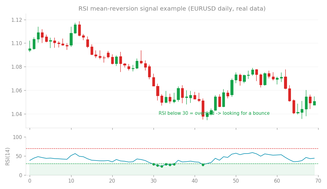
The dip buyer’s skeleton: buying oversold bounces, like the crash buyer, yet hunting different prey, as the correlation numbers show. Only 13% of signals coincide, monthly correlation sits near +0.25. Snap-back from crashes and orderly dips are different prey. That becomes the setup for the blend below.
Chapter 4: it does not travel to other markets (study 250)
How far does the edge generalize? First stop: the 26 instruments my EA actually trades, FX, metals, index CFDs.
| Class | Best variant t | PF | Verdict |
|---|---|---|---|
| FX (18 pairs) | +0.17 | 1.04 | no reversion (as predicted in advance) |
| Indices (6) | +1.37 | 1.39 | right direction, insufficient power |
| Metals (2) | +0.22 | 1.07 | rejected |
The transplant failure illuminated the edge’s true anatomy. The Monday buyer’s income is hundreds of idiosyncratic panics across 613 stocks, each on its own schedule, harvestable in cross-section. The reversion phenomenon exists faintly in indices too, but six highly correlated series crash simultaneously, so effective event count accrues only along the time axis. Neither the statistics nor the deployment opportunities ever stack up. A stock edge belongs to stocks.
Chapter 5: it does travel to other stocks (studies 251, 252)
Generalization within stocks came next: 184 freshly fetched tickers with zero overlap against the original panel, deliberately different in character (materials, banks, staples, utilities, REITs, transport), run with zero parameter choices.
The edge held: +85.8bp out of sample, t=+3.39, PF 1.36, beating the random control by +74bp at the 100th percentile. Not an artifact of stock selection. But the portfolio earned only +1.00% monthly (PF 1.93), because defensive names crash three times less often. A clean decomposition emerged: whether the edge is real, and how often it pays, are separate questions.
So, merge. On the combined 613-ticker universe, the cross-sectional stream thickened enough that even the deep -15% threshold, statistically hopeless on either universe alone, stood at t=+7.5 out of sample. The portfolio (10% per name, 10 names max, cash only) reached +4.81% monthly at PF 1.67 over the full period.
Chapter 6: making the numbers honest (study 253)
Final act: three precision passes. Every portfolio number so far came from simplified accounting that recognized profit and loss only at exit. The precise engine marks every open position to market daily.
| Setup | Monthly | PF | Max DD | Sharpe | Worst month |
|---|---|---|---|---|---|
| Monday crash buyer alone | +4.66% | 1.67 | -41.8% | 1.46 | -13.6% |
| RSI2 dip buyer alone | +3.13% | 1.47 | -44.2% | 1.40 | -25.5% |
| 50/50 blend | +4.06% | 1.51 | -17.9% | 1.79 | -13.8% |
Monthly returns barely moved, but the true max drawdown is -41.8%, not the -32.3% the simple accounting showed. The valley of unrealized losses was invisible before; I under-estimated by ten points and am saying so.
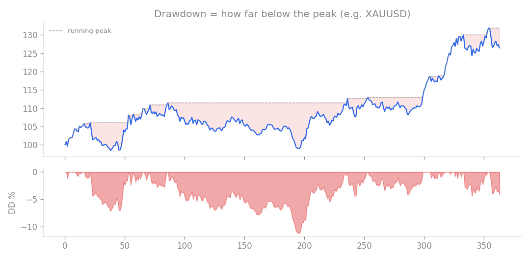
How to read drawdown: the red shading is the sag below the running peak. Mark-to-market accounting measures this valley properly, which is to say deeper.
Precision made the blend the star. The crash buyer’s worst valley is COVID, the dip buyer’s is the 2008 crisis, and at +0.25 correlation, holding both halves with monthly rebalancing shrinks the drawdown to -18%. The blend is the confirmed recommendation.
Two robustness passes closed the book. Doubling all costs to 4 cents plus 4bp leaves +3.10% monthly at PF 1.42. And the one that matters most, survivorship: this panel contains only stocks alive in 2026, so the crash buyer’s worst enemy, the stock that crashes straight into delisting, is absent by construction. Synthetic stress, forcing a fraction of entries into delisting-grade losses:
| Assumption | Monthly | PF |
|---|---|---|
| Baseline (bias ignored) | +4.66% | 1.67 |
| 0.5% of entries lose half | +3.90% | 1.53 |
| 1% go to zero | +1.71% | 1.23 |
| 2% go to zero | -1.30% (ruin) | 0.96 |
Break-even sits at 1.5 to 2% of entries going to zero. Given how rarely a large-cap loses everything inside a 3.8-day holding period (bankruptcy delistings run 0.1 to 0.3% per year), my realistic expectation lands in a +3.5% to +4.5% monthly band.
The final form, and how far to trust it
Confirmed rule: watch 613 names; buy any with a 5-day return of -10% or worse at the first close of the trading week (10% of capital per name, 10 names max); sell at the close once price recovers the 5-day SMA (10 days max). Recommended deployment: that rule blended 50/50 with the RSI2 dip buyer, monthly rebalanced: +4.06% monthly, PF 1.51, -17.9% max drawdown.
The grounds for trust: every pre-registered gate passed, the random control beaten at the 100th percentile in both periods, replication on a disjoint universe, 21 profitable years across five regimes, and survival at double costs. The discounts to apply: survivorship bias (the table above), out-of-sample decay (+211bp per trade shrank to +117bp, and may shrink further), and the fact that no real money has yet traded this. Do not read these tables as a promise.
The original Friday idea was wrong. But because the failure was measured precisely, weekday by weekday, the fix turned out to be a single day’s shift. Hypotheses are allowed to be wrong; a rig that measures exactly how they are wrong is what finds the next right answer. Of everything in these seven studies, that is the point most worth taking home.