
Weekend-gap fades alone added 30% to monthly returns
The Weekend Gap fade strategy that I previously rejected has returned as a potential candidate for my portfolio.
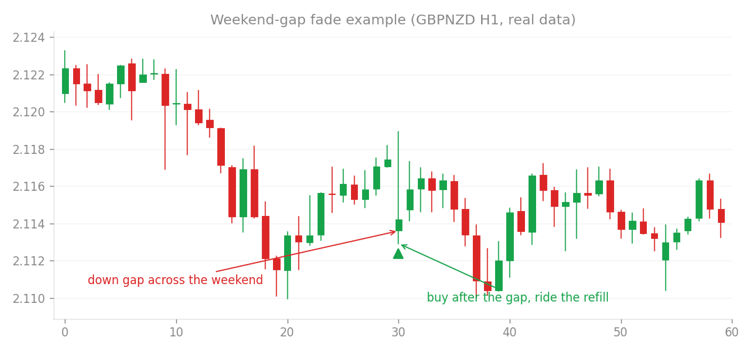
Weekend-gap fade example (GBPNZD H1, real data): trading the refill of a down gap across the weekend.
The Weekend Gap fade strategy that I previously rejected has returned as a potential candidate for my portfolio. In an earlier study, I dismissed this strategy because early market-open slippage of 2 to 5 pips caused it to collapse. However, my current implementation enters one hour after the market opens, effectively bypassing that liquidity trap.
The Strategy Logic
The strategy triggers a buy order when the market gaps down by more than 0.5 ATR on Monday morning. It exits either at the first bullish price reversal or after 12 hours. The edge here is highly specific: it relies entirely on the first hour of trading on the second H1 bar. If I delay entry by even one hour, the Profit Factor (PF) plummets from 3.25 to 0.85. In other words, this strategy profits by providing liquidity during a time of wider spreads. This makes the actual, real-world spread the ultimate judge of its success. My analysis of Dukascopy tick data across six pairs shows that at the two-hour mark, the spread is only 1.3 to 1.7 times the normal Wednesday spread. Because I wait for that first hour, I naturally avoid the initial chaotic opening where spreads can widen to 2 to 6 times the norm.
Performance and Integration
When integrated into my existing Core v1.6.0 system, the strategy provides a meaningful boost. I tested it using a conservative cost model (1.5x spread + 0.75 pip slippage) across 10 instruments.
| Configuration | PF | Monthly Return | DD | MC Pass Rate |
|---|---|---|---|---|
| Core v1.6.0 (Base) | 1.57 | +0.788% | -8.39% | 54.2% |
| + Weekend Gap (0.25% risk) | 1.65 | +0.913% | -8.01% | 63.7% |
| + Weekend Gap (0.375% risk) | 1.69 | +0.972% | -8.07% | 68.1% |
| + Weekend Gap (0.50% risk) | 1.73 | +1.028% | -8.44% | 71.9% |
| MC (Monte Carlo pass rate) represents the probability of meeting funding firm rules based on daily return resampling. | ||||
| By adding this sleeve, I achieved a 30% increase in monthly returns without increasing the drawdown. This is the largest performance gain since the v1.5.0 update and outperforms the Connors strategy integration I tested previously. |
Verdict and Next Steps
I am classifying this as a conditional candidate for deployment. Before it goes live, I need to clear four hurdles:
- Spread Calibration: I have added time-based spread logging to my EA telemetry (v1.15.0) to calibrate against my specific brokers (Purple/Axiory) because Dukascopy data is only a proxy.
- Intraday Stress: I must run an M1 intraday reconstruction to check for worst-case single-day losses during the 1 to 12-hour holding period.
- Risk Capping: My total risk at 0.5% per pair across 10 instruments (5% total) exceeds some prop firm limits. I need to implement a portfolio-level entry gate or a cap on the number of simultaneous active instruments.
- Pipeline Review: I need to recalculate how this interacts with my existing dynamic risk and flat-guard settings. While the strategy shows strong statistical significance (DSR 0.9999), the edge appears to have strengthened only since 2021. Because this is a relatively new phenomenon, I will keep a close watch on structural changes through forward monitoring and annual re-verification.
How this connects
This verification builds on earlier ones (what failed before and what I tried this time, comparisons between approaches).