Polishing the turn-of-month anomaly went nowhere
Adding a filter to avoid overbought conditions proved to be the only effective way to improve the Turn-of-the-Month (TOM) calendar strategy.
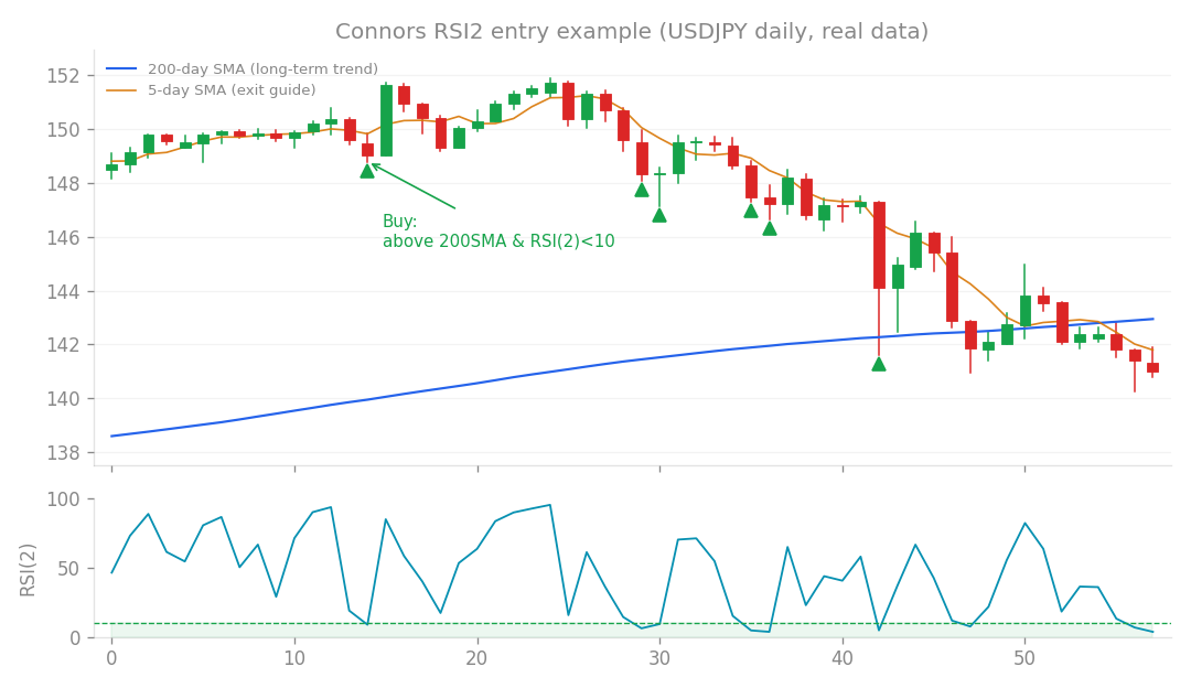
Connors RSI2 entry example (USDJPY daily, real data): buy the dip when price is above the 200-day SMA and RSI(2) falls below 10.
Adding a filter to avoid overbought conditions proved to be the only effective way to improve the Turn-of-the-Month (TOM) calendar strategy. Meanwhile, attempting to shorten the timeframe for Connors-LS strategies resulted in catastrophic performance due to transaction costs.
Testing filters for the TOM anomaly
I tested six different filters for the TOM strategy, including technical indicators like SMA200 and RSI14 as well as a subjective “support proximity” score. These were tested across seven major currency pairs on a daily timeframe with a risk per trade of 0.125%.
| Filter | IS (2015-2020H1) | OOS (2020H2-2026) |
|---|---|---|
| Baseline (No filter) | PF 1.00 / 0.000% | PF 1.24 / 0.030% |
| RSI14 <= 55 | PF 1.11 / 0.012% | PF 1.48 / 0.028% |
| The RSI14 filter was the only one that provided consistent improvement across both the in-sample (IS) and out-of-sample (OOS) periods. In other words, the strategy performs better when we avoid entering trades while the market is already overextended. The results showed a “plateau” of robustness, meaning the improvement held steady across thresholds of 50, 55, and 60. | ||
| Other filters failed to produce value. SMA200 trend filtering actually degraded performance, suggesting that the TOM effect is a flow-based anomaly that operates regardless of the broader trend. Furthermore, the subjective support proximity score failed to align between the two periods. While such manual scoring works for trend-following entries, it does not translate to flow-based anomalies. | ||
I have adopted the RSI14 <= 55 filter (setting InpCalRsiMax=55) for the new v1.8.1 version of the EA. |
Why shortening the timeframe for Connors-LS failed
I also examined whether the Connors-LS logic could be adapted from a daily timeframe (D1) to lower timeframes like H4 or H1. The results were clear:
| Timeframe | IS PF / Monthly | OOS PF / Monthly |
|---|---|---|
| D1 | PF 1.19 / 0.052% | PF 1.35 / 0.082% |
| H4 | PF 0.92 / -0.207% | PF 1.10 / 0.191% |
| H1 | PF 0.93 / -0.655% | PF 0.87 / -1.126% |
| The performance collapse on the H1 timeframe resulted in a 56% drawdown, highlighting a fundamental issue with high-frequency trading. By moving from D1 to H1, the number of trades increased by roughly 27 times. Because the expected profit per trade shrinks as you move to shorter timeframes, the total cost of spreads and commissions grew much faster than the gross profit. | ||
| In other words, increasing the trade frequency simply magnified the transaction costs until they erased the strategy’s edge. The D1 timeframe remains the lower limit where the edge is still greater than the cost. I am keeping the strategy on the D1 timeframe and rejecting the move to shorter timeframes. |
How this connects
This verification builds on earlier ones (what failed before and what I tried this time, comparisons between approaches).