Market Regime Switching: Our EA's Smart Strategy Hit a Wall!
## What's the big idea?
A beginner-friendly summary of the verification: “Market Regime Switching: Our EA’s Smart Strategy Hit a Wall!”.
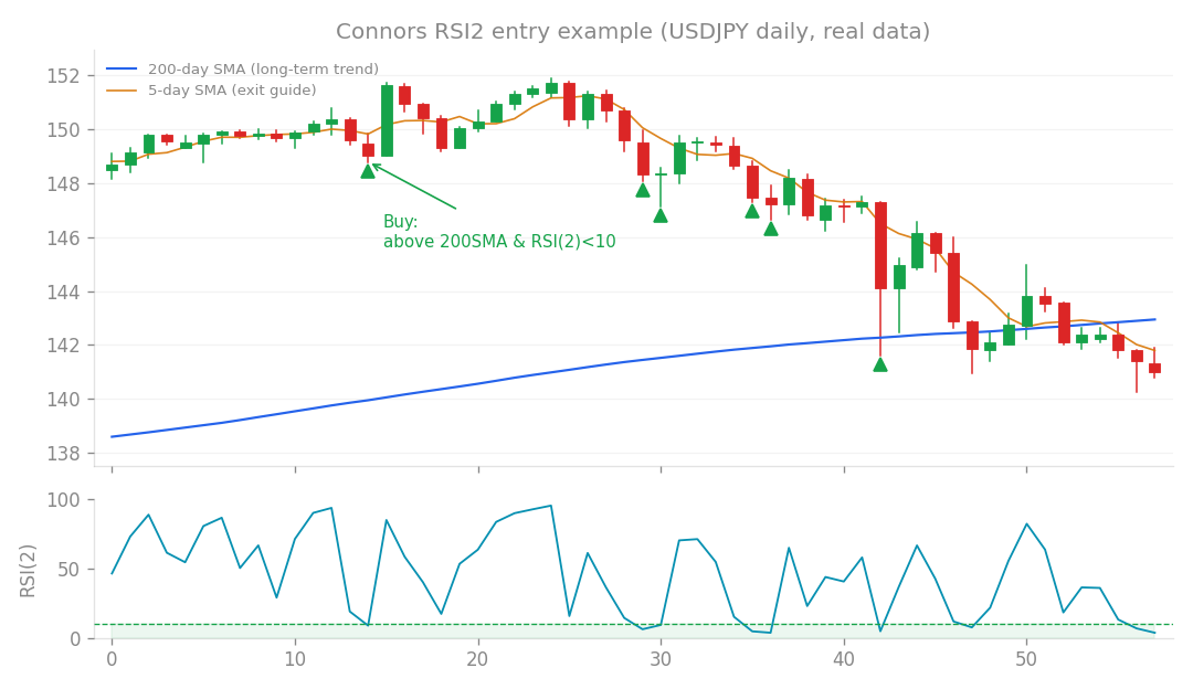
Connors RSI2 entry example (USDJPY daily, real data): buy the dip when price is above the 200-day SMA and RSI(2) falls below 10.
What’s the big idea?
We’re always looking for ways to make our algorithmic FX trading strategies (EAs) smarter. Our existing EA, version 1.5.0, is pretty solid, largely thanks to two distinct “edges” it uses. Think of an “edge” as a consistent statistical advantage in the market that helps you make profitable trades over time. One edge, which we call “Core,” thrives in trending markets – when prices are moving consistently up or down. The other, “Connors,” is designed for range-bound markets or when prices are pulling back within a trend (mean reversion). The exciting idea we wanted to test was this: what if we could dynamically allocate our trading capital between these two edges based on the current market conditions? If the market is strongly trending, we’d send more capital to “Core.” If it’s choppy or ranging, we’d favor “Connors.” This “meta-allocation” or dynamic rotation seemed like a logical step to potentially outperform a fixed 50/50 split. We hypothesized that by intelligently shifting resources, we could capture more profit than simply running both edges with a constant allocation.
How I tested it
To test this, we needed a reliable way to measure market conditions, specifically “trend strength.” For this, we used basket ADX. ADX (Average Directional Index) is a popular technical indicator that tells you how strong a trend is. A high ADX value suggests a strong trend, while a low ADX indicates a weak or range-bound market. We used a “basket” ADX, meaning we looked at the ADX across multiple currency pairs to get a broader sense of the overall market environment.
Our main goal was to see if there was a predictable relationship between market trend strength (measured by ADX) and which of our two edges was performing better. We calculated the performance “spread” between Core and Connors (Core’s profit minus Connors’ profit) and then looked at its correlation with the ADX value.
- If our hypothesis was correct: We’d expect a strong positive correlation. Higher ADX (strong trend) would mean Core performs much better than Connors.
- Alternatively: If lower ADX (range-bound) meant Connors performed better, we might see a negative correlation.
- We also did a quantile analysis, which basically means we looked at how the performance difference changed across different ADX levels (e.g., what happened when ADX was in the bottom 25% vs. top 25%).
What happened?
The results were… well, let’s just say they didn’t support our grand hypothesis!
The correlation between basket ADX and the (Core - Connors spread) was a tiny -0.035.
In other words, that’s practically zero! It means there was almost no linear relationship whatsoever between how strong the market trend was and which of our two edges was outperforming the other. The quantile analysis also showed a “non-monotonic” pattern, meaning there was no clear, consistent trend in performance differences as ADX changed.
So, the dream of predicting which edge would win based on market regime simply didn’t materialize. We couldn’t predict which strategy would be superior just by looking at trend strength.
What I learned
This outcome might seem disappointing, but it’s a fantastic learning opportunity! It reinforced some crucial lessons about strategy design and market dynamics:
- Edges Aren’t Always Mutually Exclusive: We initially thought of “Core” as purely trend-following and “Connors” as purely mean-reversion (range-bound). But the reality is more nuanced.
- “Connors” (mean reversion) can still find profitable opportunities even in a trending market by buying pullbacks during an uptrend or selling rallies in a downtrend. It’s not just for flat markets.
- Similarly, “Core” (breakout strategy) can sometimes find small, profitable breakouts even within a larger range-bound market. This means the two edges aren’t cleanly separated by market phase. They both have some degree of effectiveness across different market regimes.
- The Existing Fixed Allocation Works: Because both edges have overlapping functionality and aren’t perfectly segmented by market conditions, our existing fixed allocation in v1.5.0 is likely already doing a great job of capturing the best of both worlds. It’s not missing out on opportunities by not dynamically shifting capital.
- Dynamic Allocation Adds Timing Risk: Trying to time the market by switching between strategies based on indicators like ADX introduces additional complexity and “timing risk.” If our ADX signal is even slightly off, or if the market quickly changes character, we could end up allocating to the wrong strategy at the wrong time. This study reconfirms a finding from previous research (studies 95 and 45) that dynamic allocation often fails to beat a well-optimized fixed allocation, precisely because of this added timing risk. Ultimately, this research led us to a clear conclusion: there’s no solid foundation to implement dynamic rotation based on trend strength for these two edges. The existing version 1.5.0, with its fixed allocation, remains the optimal approach. Sometimes, the simplest solution is indeed the best!
How this connects
This verification builds on earlier ones (what failed before and what I tried this time, comparisons between approaches).