A +33.8% backtest fell to -3.0% in walk-forward: all three roads to complexity failed
Five studies on making a trading system more complex: letting machine learning dig through features, stacking indicators on fractals and across timeframes, and shrinking the timeframe. Every fixed-period winner evaporated under walk-forward testing, and the same failure pattern ran through all five.
Over the full test period the numbers read +33.8% with a PF of 1.15. For a moment I thought I had finally found it. Then the walk-forward test came back: -3.0% overall, profitable in one year out of five. Gone.
This article merges five studies (research notes 34, 44, 45, 47 and 61) into one story about complexity. I attacked the market from three directions that every trader eventually tries: let machine learning dig through a mountain of features, stack indicators on top of each other (a fractal base, fractals plus filters, then a multi-timeframe combo), and shrink the timeframe for more trades. All three roads ended in rejection. But the five studies failed in exactly the same shape, and that shape is worth more than any single result.
First time here? What you need to know
For new readers: this blog is a verification diary. I (one person) build my own automated FX trading program (an EA), statistically test trading methods, and publish everything, wins and losses alike. “Study N” refers to my numbered research log. The tests run on years of real price data for major currency pairs and gold, from 1-minute to daily bars.
Three terms. PF (profit factor) is gross profit divided by gross loss; above 1 means profitable. DD (drawdown) is the decline from an equity peak, like how far back down the mountain you have slid. And the star of this article is walk-forward testing: pick the best settings on a few years of data, then test those settings on the following unseen year, and repeat. It is the procedure that exposes settings which merely memorized the past.
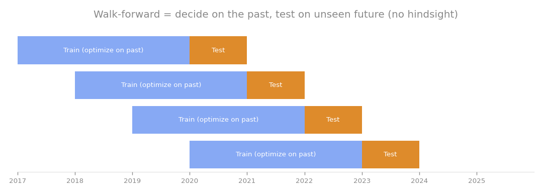
Walk-forward testing in one picture. Settings chosen on the past must answer for themselves on data they never saw. All five studies died at this gate.
Road 1: feed machine learning 19 features (study 34)
Start with the brute-force road. I fed 19 market features (moving averages, ADX, momentum and more) to a machine learning model (LightGBM) and asked it to predict price direction across a pool of 20 currency pairs. To prevent leakage, where the model accidentally peeks at the future, the walk-forward included an embargo gap between training and test windows.
| Prediction target | Result | Note |
|---|---|---|
| Next-day direction | -12.4%, 50.9% accuracy | Coin-flip territory |
| 5-day and 10-day, long and short | Loss | Short side dragged it down |
| 10-day, long only | +6.3%, DD -3.2%, 6 of 8 years | The only positive |
The only profitable configuration was long-only over a 10-day horizon. And when I inspected which features the model leaned on, they were the 200-day moving average, ADX and momentum. Trend indicators, all of them. The machine had not unearthed hidden treasure; it had rediscovered the trend-following logic I already run in plain rule-based form.
Even next-day direction came out at 50.9% accuracy. Give the most flexible method in the toolbox free rein over price data, and the only substantive edge it finds is riding the trend. Keep that sentence in mind, because it foreshadows everything below.
Road 2: stack indicators. First the fractal base collapsed (study 44)
The second road is the classic one, stacking indicators. As the base I chose the Bill Williams fractal, the well-known marker that flags a high or low when the central bar exceeds its n neighbors on both sides. I added a shift correction so the signal is only used after it has actually formed, preventing look-ahead bias.
The textbook version, symmetric long and short with no filters, was a massacre: -98% on H1, +1% on H4, -13% on D1. The hourly chart wiped the account out almost entirely.
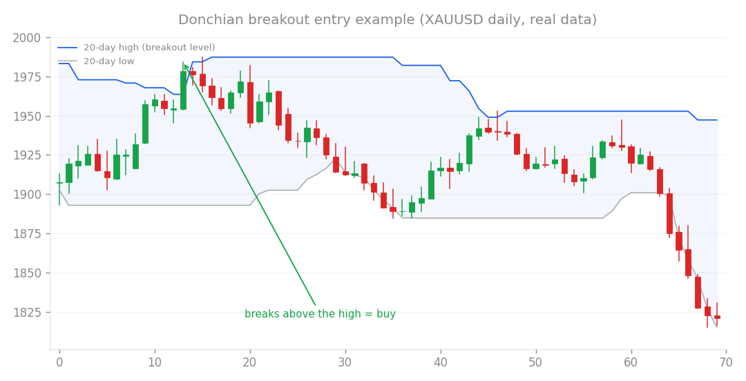
A breakout above recent highs. As it turned out, this is all a fractal really is.
So I restricted it to long-only and added a moving-average trend filter. On fixed test periods the numbers suddenly looked respectable: +13.8% on D1 with PF 1.39 and DD -5.7%, and +24.6% on H4. Then walk-forward testing dismantled it. D1 finished at -8.4% overall, profitable in 1 of 7 years. H4 finished at -5.4%, profitable in 3 of 7.
The autopsy delivered the verdict. Daily correlation between this fractal system and my deployed trend-following core measured 0.83. Fractals were not finding new information. They were detecting swing highs and lows, which makes them a reinvention of the Donchian channel, the classic highest-high breakout method. No independent edge, just a familiar one wearing a different name.
Still stacking: fractals times RSI times ADX (study 45)
Maybe a weak base can be stabilized by more filters? I wondered the same thing. So I added RSI (an overheat gauge) and ADX (a trend-strength gauge) to the fractal system, alone and in combination, eight variants in total, and ran them all through walk-forward testing.
Total wipeout. My robustness bar was simple: positive overall and profitable in at least 5 of 7 years. None of the eight variants cleared it. The best one managed 4 of 7 winning years on H4 with a total return of roughly zero. Even combinations that had looked brilliant on fixed periods, like fractals with RSI below 70 showing over 50% growth, were no exception.
The way they degraded is the interesting part. Every added filter cut the trade count, and numbers that looked great at first sank toward average as the testing widened. When the over-optimization (curve-fitting to a specific slice of the past) was removed, the edge went with it, because there had never been an edge underneath. Parts with zero edge sum to zero no matter how many you stack.
The summit of stacking: RSI plus SMA across timeframes (study 47)
The final form of the stacking road was multi-timeframe (MTF) analysis, combining charts of different resolutions. A higher-timeframe moving average defines the big picture, a lower-timeframe moving average confirms the trend, and RSI times the pullback entry. Three layers of confirmation. I tested four timeframe pairings with 36 parameter combinations each, with strict resampling and shifting so no higher-timeframe bar is used before it closes.
| Test | Result |
|---|---|
| Fixed-period optimum (H1 base + H4) | +33.8%, PF 1.15 |
| Fixed-period optimum (H4 base + D1) | +15.5%, PF 1.11 |
| Walk-forward (train 3 years, test 1) | -3.0% overall, 1 of 5 years |
| Best fixed settings applied to other pairs | -11.0% overall, 2 of 6 pairs positive |
This is where the opening numbers came from. The +33.8% optimum turned into -3.0% the moment it faced unseen data. Worse, the chosen parameters flailed between windows, the SMA period flipping between 100 and 200, the RSI buy level between 30 and 50. A forecaster who changes his story every time is not describing a stable law, and neither was this system.
One small consolation survived. Walk-forward drawdowns stayed shallow, between 0 and -7% each year. So the combo is a “no edge but low risk” machine. That leaves it a candidate for a diversification slot in a portfolio someday, but it is not a source of profit.
Road 3: shrink the timeframe (study 61)
The third road is less about adding parts and more about speeding up. If a strategy wins on the hourly chart, would faster charts mean more trades and more profit? I took my deployed breakout logic, kept every parameter identical, and walked it down from H1 to M30, M15 and M5 (2019 to 2025, per-symbol spreads included).
| Timeframe | Return | PF | Winning years | Max DD |
|---|---|---|---|---|
| H1 (baseline) | +31% | 1.36 | 5/5 | -8.6% |
| M30 | +37% | 1.19 | 5/5 | -16.2% |
| M15 | +13% | 1.02 | 4/5 | |
| M5 | -77% | 0.76 | 0/5 | -85% |
Trades ballooned from 1,428 on H1 to 18,755 on M5. But the only thing that multiplied was the number of times I paid the spread. PF and DD degraded monotonically, and the symmetric Donchian variant did even worse, finishing M5 at -100%, a total loss, with the short side crushed by costs and false signals.
Then I stress-tested slippage (the gap between the ordered and executed price). M5 was dead under any assumption, PF sliding from 0.76 to 0.48. M15 was profitable only in a fantasy world of zero slippage: adding just 0.5 pips pushed PF from 1.02 to 0.96, under water. M30 was the only lower timeframe with any tolerance, surviving 1 pip (PF 1.19 to 1.10), yet it remains a strictly degraded H1, with PF down from 1.36 to 1.19 and drawdown nearly doubled from -8.6% to -16.2%. Nothing improved by going faster. Nothing.
The shape all five failures share
Line the studies up and the pattern is unmistakable.
- Fixed-period tests always produce attractive numbers (+13.8%, over +50%, +33.8%)
- Walk-forward testing erases them (-8.4%, roughly zero, -3.0%)
- The post-mortem finds either a rediscovery of the known trend edge or plain curve-fitting
The machine learning model dug up trend indicators. The fractal correlated 0.83 with my trend core, a Donchian channel in costume. The multi-timeframe optimum was over-optimization with parameters that danced between windows. The shorter timeframes just fed the spread. Complexity created no new edge anywhere. What it created, reliably, was performance that looks real on a fixed window and cannot survive contact with the future.
So what does work? From where I stand now, after many more studies since these five, the only substantive edge price data has yielded is a simple structure: ride the trend on slower timeframes. And because the complexity search ended in rejection across the board, I can hold that conclusion without the nagging doubt of “maybe I just haven’t tried the fancy version yet”. A negative result is a survey marker. It fixes the words “nothing buried here” onto the map, permanently.
This article consolidates studies 34, 44, 45, 47 and 61.